Analyses of MD trajectories
a simple tutorial to analyse your MD trajectory with Gromacs
WORK IN PROGRESS! Please, wait ‘till this page is completed!
The Molecular Dynamics (MD) trajectory will be analyzed using the modules contained in the Gromacs 2023 suite. This part of the tutorial can be performed directly on a server or locally on your own PC, where Gromacs must be installed.
If Gromacs is installed, simply run the command gmx -version to check which version is installed. If it is not installed, you can install it using the command sudo apt-get install -y gromacs.
Step 1: retrieve the structure
The file must be prepared for subsequent analyses by fitting the trajectory. Rotational and translational movements must be removed. Removing rotational and translational movements from a molecular dynamics trajectory focuses the analysis on the internal dynamics of the system. This ensures that calculated metrics like RMSD reflect changes in the molecule's shape and internal structure, rather than its overall position or orientation.
For the purposes of this tutorial, the fitting will be performed on the entire protein without its hydrogens. This can be done using the command:
gmx trjconv -s yourfile_nowat.pdb -f your_trajectory.xtc -fit progressive -o your_trajectory_fitted.xtc
where:
- -s specificies the reference structure;
- -fspecifies the input trajectory;
- -fit instructs Gromacs to do a progressive fit in which the first timeframe is fitted to the reference structure in the structure file to obtain and each subsequent timeframe is fitted to the previously fitted structure;
- -o specifies the name of the output
Once the command is executed, select Protein-H as the group to fit the trajectory by typing 2, and System as the group to write the output trajectory by typing 0. You can visualize the difference between the trajectory fitted and not fitted using VMD!


Step 2: installation of Xmgrace
To visualize the resulting files from the analyses performed with Gromacs, you will need to install xmgrace. Xmgrace is a scientific plotting tool for creating high-quality graphs and visualizations. It is widely used in the scientific community for plotting data from molecular dynamics simulations and other types of scientific data.
From the command line, simply type:
sudo apt-get install grace
For more information, visit the Xmgrace manual.
Step 3: Root Mean Square Deviation (RMSD)
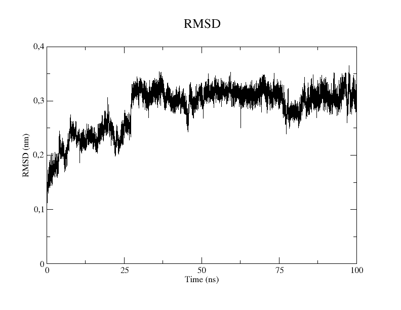
RMSD (Root Mean Square Deviation) is a measure used to quantify the difference between two three- dimensional structures of a molecule. It is calculated as the square root of the average of the squared distances between corresponding atoms in the two structures. RMSD is often used for evaluating structural stability, comparing conformations or studying conformational transitions. Usually a typical output should have on the x-axis the simulation time. On the y-axis, there is the RMSD value expressed in nm.
Typically, the curve shows a rapid increase in the early part of the simulation, then stabilizes around a value and oscillates around it. This means that the simulation took the initial part of the time to complete equilibration, then reached a stable phase called a plateau or convergence.
For the purposes of this tutorial, the RMSD will be calculated on the entire protein without the hydrogens. To calculate the RMSD, use the command:
gmx rms -s your_file.pdb -f your_trajectory_fitted.xtc -tu ns -o rmsd.xvg
where:
- -s specificies the reference structure;
- -fspecifies the input trajectory;
- -tu ns intructs Gromacs to convert picoseconds to nanosecond. The time in the output will be written in ns;
- -o specifies the name of the output
Once the command is executed, select Protein-H as the reference group by typing 2, and Protein-H as the group to calculate the RMSD with by typing 2.
You will retrieve a rmsd.xvg that can be opened using the command:
xmgrace rmsd.xvg 
Step 4: Root Mean Square Fluctuations (RMSF) Once the command is executed, select Protein-H as the reference group to calculate RMSF by typing 2. You will retrieve a rmsf.xvg that can be opened using the command: Step 5: Principal Component Analysis (PCA)
RMSF (Root Mean Square Fluctuation) is a measure used to quantify the flexibility or mobility of each atom in a molecule throughout a MD simulation. It is calculated as the square root of the average of the squared fluctuations of each atom's position relative to its average position in the trajectory.
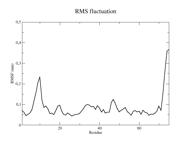
RMSF is often used for identifying flexible regions in proteins, such as loop regions or protein-ligand binding sites. The N and C-terms are a lot flexible, as shown in figure for N-terminal part.
A typical output plot of RMSF shows on the x-axis the residue index or number, and on the y-axis, the RMSF value expressed in nm.
For the purposes of this tutorial, RMSF will be calculated for each residue of the protein without the hydrogens. To calculate RMSF, use the command:gmx rmf -s your_file.pdb -f your_trajectory_fitted.xtc -res -o rmsf.xvg
xmgrace rmsf.xvg

PCA (Principal Component Analysis) is a statistical method used to identify and analyze the major patterns in the variations of a dataset. In the context of MD simulations, PCA is often used to identify the principal motions of a biomolecule. In PCA, eigenvalues and eigenvectors are fundamental concepts for understanding the major modes of variation in the data.
In PCA applied to MD trajectories, the eigenvectors of the covariance matrix represent the major modes of variation in the positions of atoms over time. The eigenvalues indicate how much each principal component contributes to the overall variance of the trajectory. These concepts are fundamental for understanding and interpreting the results of PCA and for identifying the major modes of molecular motion.
From a PCA analysis, important files to retrieve are:
- 2d projections (2dprojection.xvg) : shows the projections of the trajectories onto the principal components (PC1 and PC2);
- Collective motions (collectivemotions1.pdb, collectivemotions2.pdb, collectivemotions3.pdb) : shows the important motions of the examined system.
To perform PCA, use the command:
gmx trjconv -s your_file.pdb -f your_trajectory_fitted.xtc -skip 10 -o traj_fitted_skip10.xtcwhere:
- -skip 10 : is useful to light the trajectory and to allow a faster calculation: every 10 frames of the original trajectory, a frame is written in the output trajectory.
gmx covar -s myfile.pdb -f traj_fitted_skip10.xtc -o eigenval.xvg -v eigenvec.trr -l PCA.log -av average_PCA.pdb -tu nswhere:
- -o eigenval.xvg: specifies the output file name where the eigenvalues will be saved in XVG format;
- -v eigenvec.trr: specifies the output file name where the eigenvectors will be saved in TRR format;
- -l PCA.log: specifies the output log file name where information about the principal component analysis (PCA) will be saved;
- -av average_PCA.pdb: specifies the output file name where the average structure (average of all conformations in the trajectory) will be saved in PDB format;
- -tu ns: specifies the time unit as nanoseconds.
For all information about Gromacs 2023, please visit the manual. Thanks to Alessia Pinto for beta-testing and debugging this tutorial!
WORK IN PROGRESS! Please, wait 'till this page is completed!